DIANE Programming Interface
Source:vignettes/DIANE_Programming_Interface.Rmd
DIANE_Programming_Interface.RmdWhy an application programming interface?
In addition to the Graphical User Interface, DIANE also comes with all it’s server-side functions. They can be called from any R environment or scripts, after loading DIANE.
Using DIANE’s functions outside of the interface can be an interesting option for several reasons, among which :
It allows more flexibility and additional user-specific R analysis
It can be part of an automated pipeline
We present in this document how to use those functions on our demo data.
Input data
DIANE’s companion dataset is meant to illustrate its functionalities and provide an explicit example of the expected input data.
The chosen dataset contains the transcriptome of Arabidopsis thaliana plants exposed to global warming related conditions. It was generated for the article “Molecular plant responses to combined abiotic stresses put a spotlight on unknown and abundant genes”, by Sewelam et Al. in Journal of experimental Botany, 2020. (https://academic.oup.com/jxb/advance-article/doi/10.1093/jxb/eraa250/5842162#204457392).
The experimental perturbations studied are heat, salinity and drought in culture soil. Each factors have two levels, one of them considered as the reference, and the other one as the stress level.
To use DIANE’s functions on your data, you should provide R variables that describe your dataset the following formats.
Raw expression counts
It must be an R dataframe with gene IDs as rownames, and condition_replicate as columns. It contains row or normalized expression levels.
In order for your input to be compatible with the proposed organisms for GO terms and annotation, it should contain gene IDs as follow :
For Arabidopsis thaliana : TAIR IDs (ex: AT1G01020, or AT1G01020.1)
For Human : ensembl IDs (ex: ENSG00000005513)
For Mus musculus : ENSMUSG00000087910
For Drosophilia : FBgn0000036
For C. elegans : WBGene00000042
For Lupinus albus : Lalb_Chr00c02g0404151
For E-coli : acpS
Our demo data have raw counts presented as follow :
kable(head(abiotic_stresses$raw_counts))| C_1 | C_2 | C_3 | S_1 | S_2 | S_3 | M_1 | M_2 | M_3 | H_1 | H_2 | H_3 | SM_1 | SM_2 | SM_3 | SH_1 | SH_2 | SH_3 | MH_1 | MH_2 | MH_3 | SMH_1 | SMH_2 | SMH_3 | |
|---|---|---|---|---|---|---|---|---|---|---|---|---|---|---|---|---|---|---|---|---|---|---|---|---|
| AT1G01010.1 | 127.0 | 67.9 | 65.5 | 94.0 | 88.1 | 95.9 | 65.1 | 100.3 | 126.8 | 95.4 | 135.0 | 117.2 | 96.7 | 104.4 | 98.1 | 94.7 | 96.1 | 101.3 | 82.8 | 107.4 | 97.1 | 100.1 | 96.7 | 121.8 |
| AT1G01020.1 | 207.9 | 220.8 | 186.8 | 192.5 | 225.1 | 197.8 | 234.2 | 196.9 | 179.4 | 312.9 | 366.0 | 318.0 | 169.0 | 179.6 | 186.5 | 340.8 | 352.6 | 345.0 | 331.2 | 315.8 | 327.5 | 267.7 | 313.7 | 319.3 |
| AT1G01030.1 | 32.7 | 34.4 | 55.8 | 33.6 | 15.9 | 31.3 | 21.4 | 29.8 | 33.5 | 47.7 | 39.0 | 51.1 | 25.2 | 31.2 | 34.4 | 61.0 | 65.5 | 61.2 | 45.0 | 36.2 | 55.9 | 46.0 | 42.7 | 56.8 |
| AT1G01040.2 | 859.3 | 978.8 | 988.6 | 897.6 | 837.9 | 948.6 | 948.8 | 903.2 | 990.1 | 798.3 | 701.1 | 902.9 | 894.6 | 880.3 | 837.2 | 782.6 | 776.4 | 698.0 | 843.3 | 810.2 | 777.7 | 807.2 | 786.0 | 853.7 |
| AT1G01050.1 | 846.8 | 840.2 | 837.2 | 836.1 | 818.8 | 792.2 | 802.0 | 761.4 | 719.9 | 922.2 | 969.3 | 930.8 | 866.9 | 805.2 | 840.1 | 895.2 | 783.2 | 849.5 | 690.0 | 702.8 | 717.8 | 835.8 | 969.3 | 837.2 |
| AT1G01060.1 | 658.2 | 698.8 | 636.5 | 532.7 | 411.0 | 519.7 | 741.6 | 782.2 | 877.7 | 36.7 | 20.8 | 20.5 | 857.6 | 853.0 | 878.4 | 29.5 | 39.6 | 19.1 | 33.7 | 39.9 | 16.7 | 49.0 | 33.7 | 26.0 |
Experimental design
This is optional, and only used to fit Poisson Generalized linear models to gene clusters. It is shown here to explain our companion dataset.
For each condition name, the level of the factors corresponding to that condition in your study are to be provided.
The experiement we chose for our demo included 3 factors, heat stress (H), mannitol stress(M), as well as salinity stress (S).
You should first identify which level of each factor can be considered as the control level, and which is a perturbation. In our demo, the control condition is referred to as C. Then, the perturbation are specified by their corresponding letter, from simple to triple stress combination. For example, SH corresponds to salt and heat stresses in the control level of mannitol. As a consequence, its levels would be 1,0,1.
The design file is thus a matrix with condition names as rownames, and factor names as columns:
kable(abiotic_stresses$design)| Salt | Mannitol | Heat | |
|---|---|---|---|
| C | 0 | 0 | 0 |
| H | 0 | 0 | 1 |
| S | 1 | 0 | 0 |
| M | 0 | 1 | 0 |
| SM | 1 | 1 | 0 |
| SH | 1 | 0 | 1 |
| MH | 0 | 1 | 1 |
| SMH | 1 | 1 | 1 |
Gene annotation
We provided gene description for Arabidopsis :
kable(tail(gene_annotations[["Arabidopsis thaliana"]], n = 10))| label | description | |
|---|---|---|
| AT3G19580 | ZF2 | Encodes zinc finger protein. mRNA levels are upregulated in response to ABA, high salt, and mild desiccation. The protein is localized to the nucleus and acts as a transcriptional repressor. |
| AT5G43170 | ZF3 | Encodes zinc finger protein. mRNA levels are elevated in response to high salinity and low temperature. The protein is localized to the nucleus and acts as a transcriptional repressor. |
| AT4G24470 | ZIM | ZIM is a putative transcription factor containing an atypical GATA-type zinc-finger motif. |
| AT2G48020 | ZIF2 | Encodes a zinc transporter ZIF2. Expression of ZIF2 is regulated by alternative splicing. |
| AT5G59520 | ZIP2 | encodes a metal ion transporter whose expression is regulated by copper. |
| AT5G65930 | ZWI | encodes a novel member of the kinesin superfamily of motor proteins. recessive mutations have reduced number of trichome branches. |
| AT2G01210 | ZAR1 | ZAR1 encodes a plasma membrane localized leucine-rich repeat receptor-like kinase (LRR-RLK) that contains a putative CaM-binding domain and a Gβ |
| AT5G61350 | CAP1 | Encodes a membrane-localized receptor-like kinase that regulates root hair tip growth by maintaining cytoplasmic Ca2+ gradients. Knockouts of CAP1 produced more cytoplasmic NH4+ and ceased growth of root hairs on MS medium except when NH4+ was depleted |
| AT2G25095 | AT2G25095 | Encodes a microRNA that targets several SPL family members, including SPL3,4, and 5. By regulating the expression of SPL3 (and probably also SPL4 and SPL5), this microRNA regulates vegetative phase change. MicroRNAs are regulatory RNAs with a mature length of ~21-nucleotides that are processed from hairpin precursors by Dicer-like enzymes. MicroRNAs can negatively regulate gene expression by attenuating translation or by directing mRNA cleavage.Mature sequence: UGACAGAAGAGAGUGAGCAC. Pri-mRNA coordinates for MIR156a (converted to TAIR10 based on PMID19304749): Chr2: 10677064-10673957 (reverse), length: 3108 bp |
| AT4G31877 | AT4G31877 | Encodes a microRNA that targets several SPL family members, including SPL3,4, and 5. By regulating the expression of SPL3 (and probably also SPL4 and SPL5), this microRNA regulates vegetative phase change. MicroRNAs are regulatory RNAs with a mature length of ~21-nucleotides that are processed from hairpin precursors by Dicer-like enzymes. MicroRNAs can negatively regulate gene expression by attenuating translation or by directing mRNA cleavage.Mature sequence: UGACAGAAGAGAGUGAGCAC. Pri-mRNA coordinates for MIR156c (converted to TAIR10 based on PMID19304749): Chr4: 15415873-15413295 (reverse), length: 2580 bp |
This is not required, but it can be convenient to use this information when displaying lists of genes, to have their associated meaning.
The annotations for other organisms known to DIANE can be retrieved for any list of genes as follows :
knitr::kable(get_gene_information(c("WBGene00000013", "WBGene00000035"), organism = "Caenorhabditis elegans"))
#> | label | description | |
|---|---|---|
| WBGene00000013 | abf-2 | Antibacterial factor-related peptide 2 |
| WBGene00000035 | ace-1 | Acetylcholinesterase 1 |
Data pre-processing
Visualization of raw counts
For each condition, we can visualize the distributions of gene counts with boxplots or distributions. To display the distributions, you can use the argument boxplot = FALSE.
DIANE::draw_distributions(abiotic_stresses$raw_counts, boxplot = TRUE)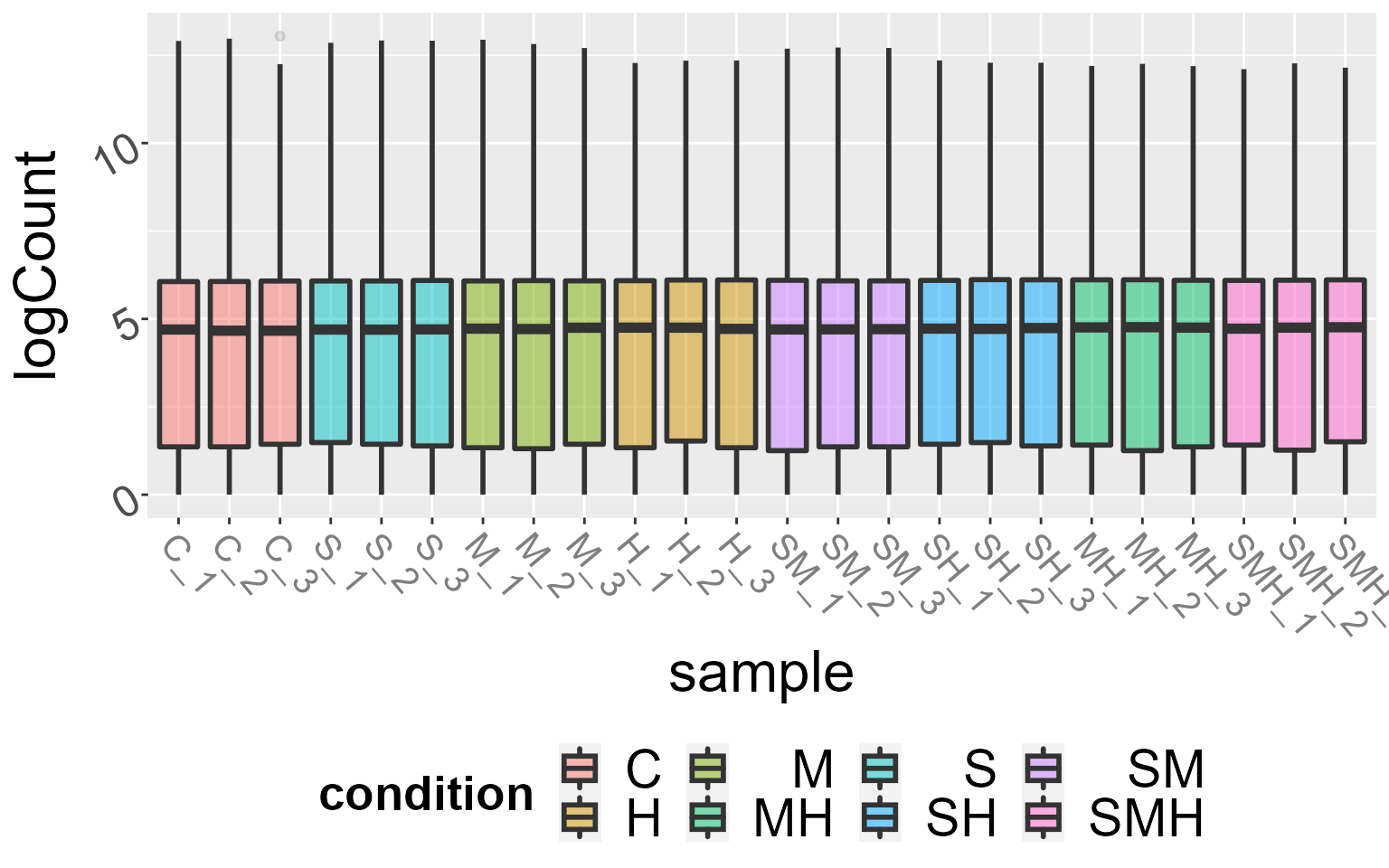
Normalization
The TCC R package is used for the normalization step here, to make samples comparable by correcting for their differences in sequencing depths. This step is mandatory before further statistical analysis.
You can choose to normalize using the methods implemented in edgeR, referenced as ‘tmm’, or the one used in DESeq, referenced as ‘deseq2’.
Those normalization methods rely on the hypothesis that a very small proportion of genes are differentially expressed between your samples. If you suspect a lot of genes could be differentially expressed in your data, TCC offers the possibility to proceed to a first detection of potential differentially expressed genes, to remove them, and then provide a final less biased normalization.
In that case, enable “prior removal of deferentially expressed genes”. TCC will perform the following setp, depending on the normalization method you chose :
+ tmm/deseq2 temporary normalization
+ potential DEG identification and removal using edgeR test method
+ tmm/deseq2 definitive normalization
We use here the default parameters (no prior removal of differentially expressed genes, and TMM method) :
tcc_object <- DIANE::normalize(abiotic_stresses$raw_counts, norm_method = 'tmm', iteration = FALSE)Note : here, our data should not be normalized, as it is already given as TPMs. Normalization is shown for the purpose of demonstration.
Low counts removal
Removing genes with very low abundance is a common practice in RNA-Seq analysis pipelines for several reasons :
- They have little biological significance, and could be caused either by noise or mapping errors.
- The statistical modeling we are planning to perform next is not well suited for low counts, as they make the mean-variance relationship harder to estimate.
There is no absolute and commonly accepted threshold value, but it is recommended to allow only genes with more than 10 counts per sample in average. DIANE thus proposes a threshold at 10*sampleNumber, but feel free to experiment with other values depending on your dataset and intensions.
threshold = 10*length(abiotic_stresses$conditions)
tcc_object <- DIANE::filter_low_counts(tcc_object, threshold)
normalized_counts <- TCC::getNormalizedData(tcc_object)
We can see the difference with the violin plot view of the effect of low count genes removal :
pre_process <- DIANE::draw_distributions(abiotic_stresses$raw_counts, boxplot = FALSE) + ggtitle("Before")
post_process <- DIANE::draw_distributions(normalized_counts, boxplot = FALSE)+ ggtitle("After")

gridExtra::grid.arrange(pre_process, post_process, ncol = 2)
#> Picking joint bandwidth of 0.411
#> Picking joint bandwidth of 0.247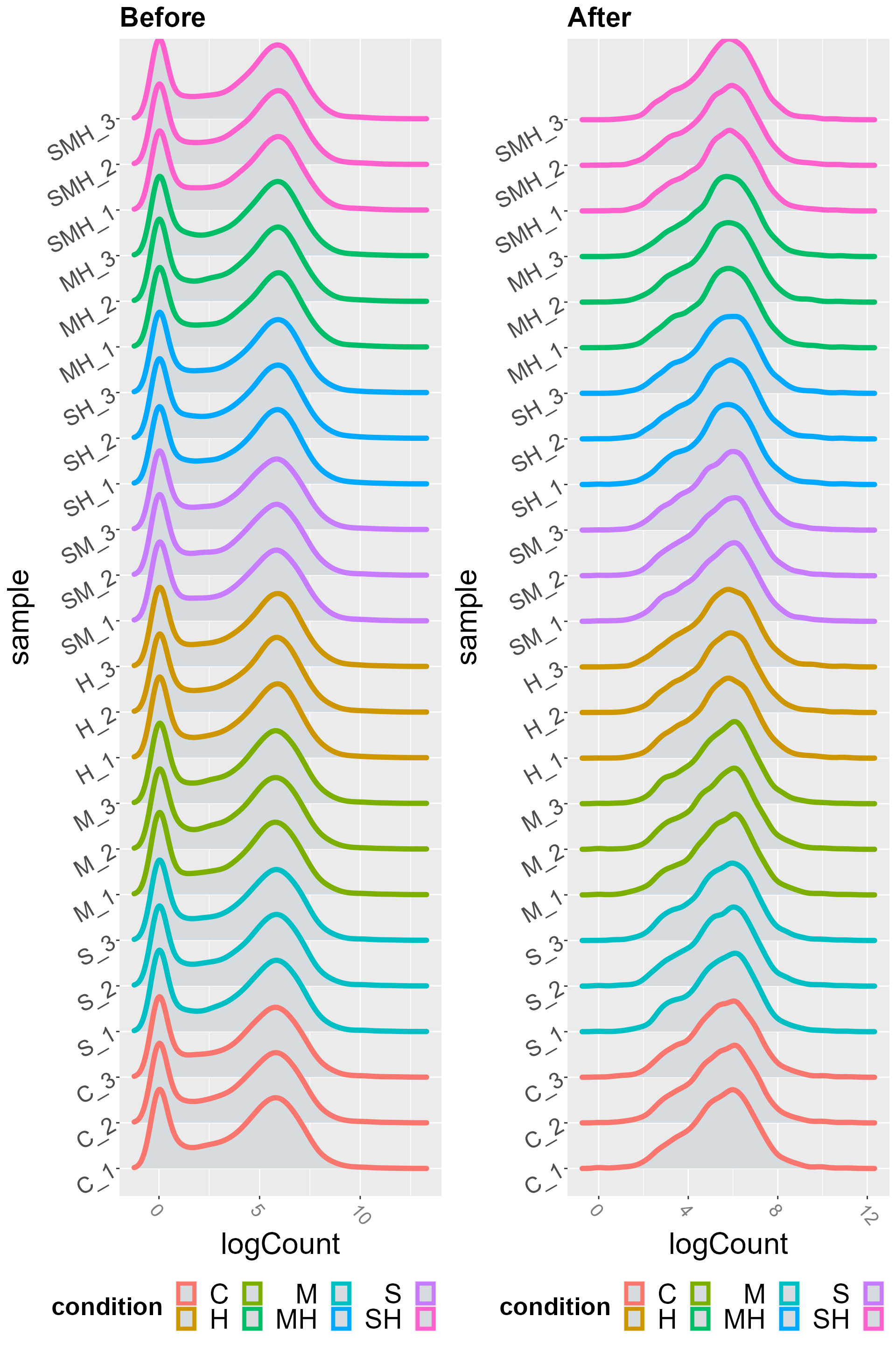
genes <- sample(abiotic_stresses$heat_DEGs,4)
DIANE::draw_expression_levels(abiotic_stresses$normalized_counts, genes = genes)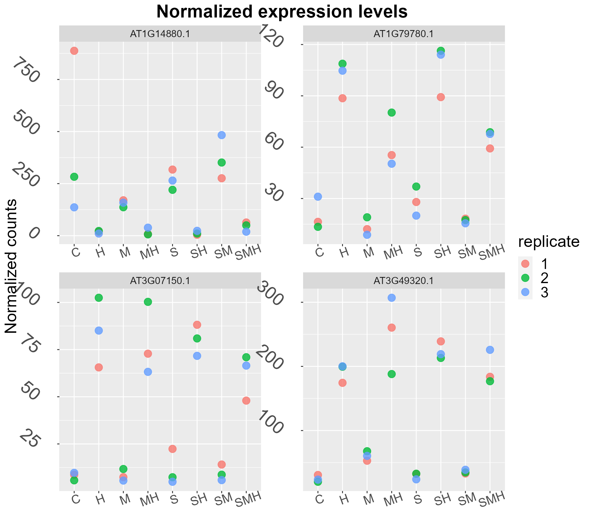
Sample homogeneity and global analysis
Principal component analysis
Performing PCA on normalized RNA-Seq counts can be really informative about the conditions that impact gene expression the most. During PCA, new variables are computed, as linear combinations of your initial variables (e.g. experimental conditions). Those new variables, also called principal components, are designed to carry the maximum of the data variability.
We can plot the correlations of the initial variables to the principal components, to see which ones contribute the most to those principal components, and as a consequence, to the overall expression changes.
Each principal component explains a certain amount of the total variability, and those relative percentages are shown in what is called the screeplot.
DIANE::draw_PCA(data = normalized_counts)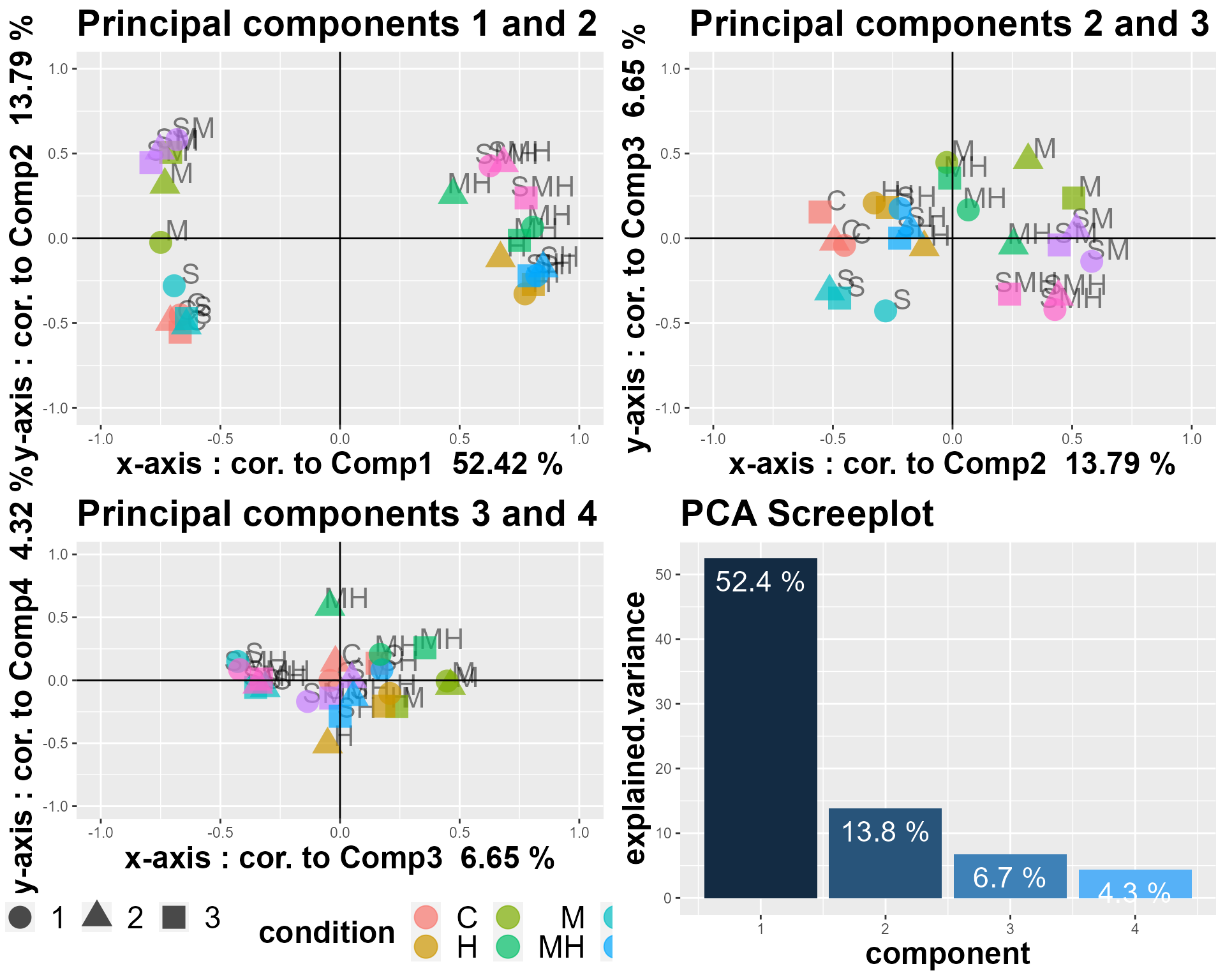
The first plane, showing the first two components, is striking in the sense that the conditions are segregated by their heat level. Indeed, we find here that 57.3% of gene expression variability can be linked to heat stress.
The second principal axis, is more correlated to osmotic stress, as conditions with mannitol stress are opposed along this axis, carrying 12.2% of gene expression variance.
Differential expression analysis
Let’s say we want to preform differential expression analysis between the conditions C and H, to get genes responding to a simple heat stress :
fit <- DIANE::estimateDispersion(tcc = tcc_object, conditions = abiotic_stresses$conditions)
#> Warning in edgeR::DGEList(counts = tcc$count, lib.size = tcc$norm.factors, :
#> norm factors don't multiply to 1
topTags <- DIANE::estimateDEGs(fit, reference = "C", perturbation = "H", p.value = 0.01, lfc = 2)

# adding annotations
DEgenes <- topTags$table
DEgenes[,c("name", "description")] <- gene_annotations$`Arabidopsis thaliana`[
  match(get_locus(DEgenes$genes, unique = FALSE), rownames(gene_annotations$`Arabidopsis thaliana`)),
  c("label", "description")]

knitr::kable(head(DEgenes, n = 10))| genes | logFC | logCPM | LR | PValue | FDR | name | description | |
|---|---|---|---|---|---|---|---|---|
| AT4G12400.2 | AT4G12400.2 | 7.756985 | 7.564179 | 2272.130 | 0 | 0 | HOP3 | Encodes one of the 36 carboxylate clamp (CC)-tetratricopeptide repeat (TPR) proteins (Prasad 2010, Pubmed ID: 20856808) with potential to interact with Hsp90/Hsp70 as co-chaperones. |
| AT5G48570.1 | AT5G48570.1 | 7.067740 | 8.853736 | 1970.131 | 0 | 0 | ROF2 | Encodes one of the 36 carboxylate clamp (CC)-tetratricopeptide repeat (TPR) proteins (Prasad 2010, Pubmed ID: 20856808) with potential to interact with Hsp90/Hsp70 as co-chaperones. |
| AT5G12110.1 | AT5G12110.1 | 5.939006 | 7.952267 | 2202.123 | 0 | 0 | AT5G12110 | elongation factor 1-beta 1 |
| AT5G64510.1 | AT5G64510.1 | 5.879518 | 6.067228 | 2228.044 | 0 | 0 | TIN1 | Encodes Tunicamycin Induced 1(TIN1), a plant-specic ER stress-inducible protein. TIN1 mutation affects pollen surface morphology. Transcriptionally induced by treatment with the N-linked glyclsylation inhibitor tunicamycin. |
| AT2G19310.1 | AT2G19310.1 | 4.212070 | 7.686615 | 1389.691 | 0 | 0 | HSP18.5 | HSP20-like chaperones superfamily protein |
| AT2G29500.1 | AT2G29500.1 | 7.731411 | 9.482692 | 1260.703 | 0 | 0 | HSP17.6B | HSP20-like chaperones superfamily protein |
| AT4G25200.1 | AT4G25200.1 | 9.148324 | 7.804942 | 1248.861 | 0 | 0 | HSP23.6-MITO | AtHSP23.6-mito mRNA, nuclear gene encoding mitochondrial |
| AT1G07350.1 | AT1G07350.1 | 3.487824 | 7.417268 | 1204.945 | 0 | 0 | SR45A | Encodes a serine/arginine rich-like protein, SR45a. Involved in the regulation of stress-responsive alternative splicing. |
| AT3G24100.1 | AT3G24100.1 | 4.107079 | 6.487794 | 1145.808 | 0 | 0 | BIA | Encodes a secreted peptide that enhances stress indued cell death. |
| AT2G26150.1 | AT2G26150.1 | 6.734306 | 6.023919 | 1110.311 | 0 | 0 | HSFA2 | member of Heat Stress Transcription Factor (Hsf) family. Involved in response to misfolded protein accumulation in the cytosol. Regulated by alternative splicing and non-sense-mediated decay. |
# plots
tags <- DIANE::estimateDEGs(fit, reference = "C", perturbation = "H", p.value = 1)
DIANE::draw_DEGs(tags)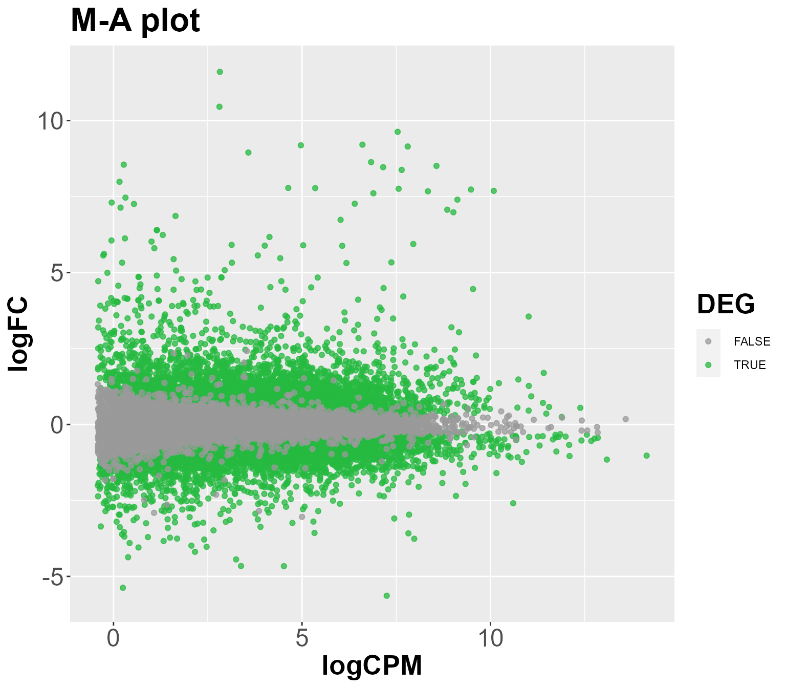
DIANE::draw_DEGs(tags, MA = FALSE)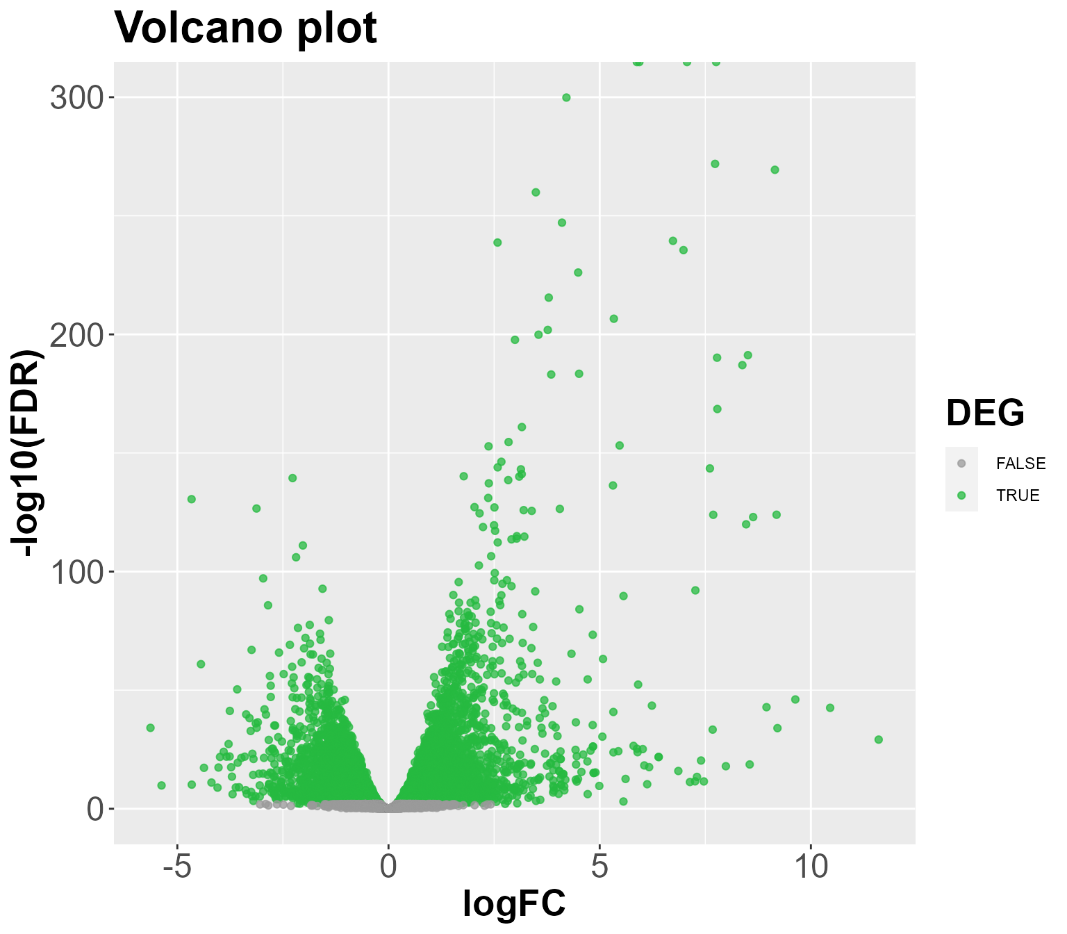
genes <- topTags$table$genes

DIANE::draw_heatmap(normalized_counts, subset = genes,
                    title = "Log expression for DE genes under heat stress")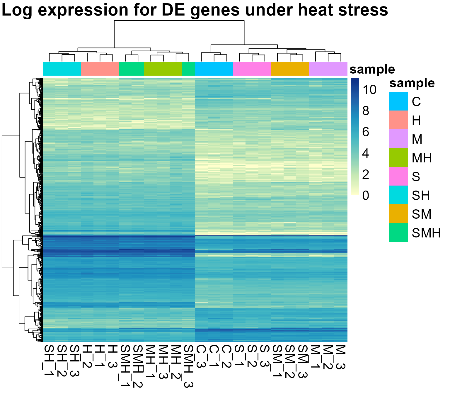
# if we only want the conditions used for differential expression analysis :
DIANE::draw_heatmap(normalized_counts, subset = genes,
                    title = "Log expression for DE genes under heat stress",
                    conditions = c("C", "H"))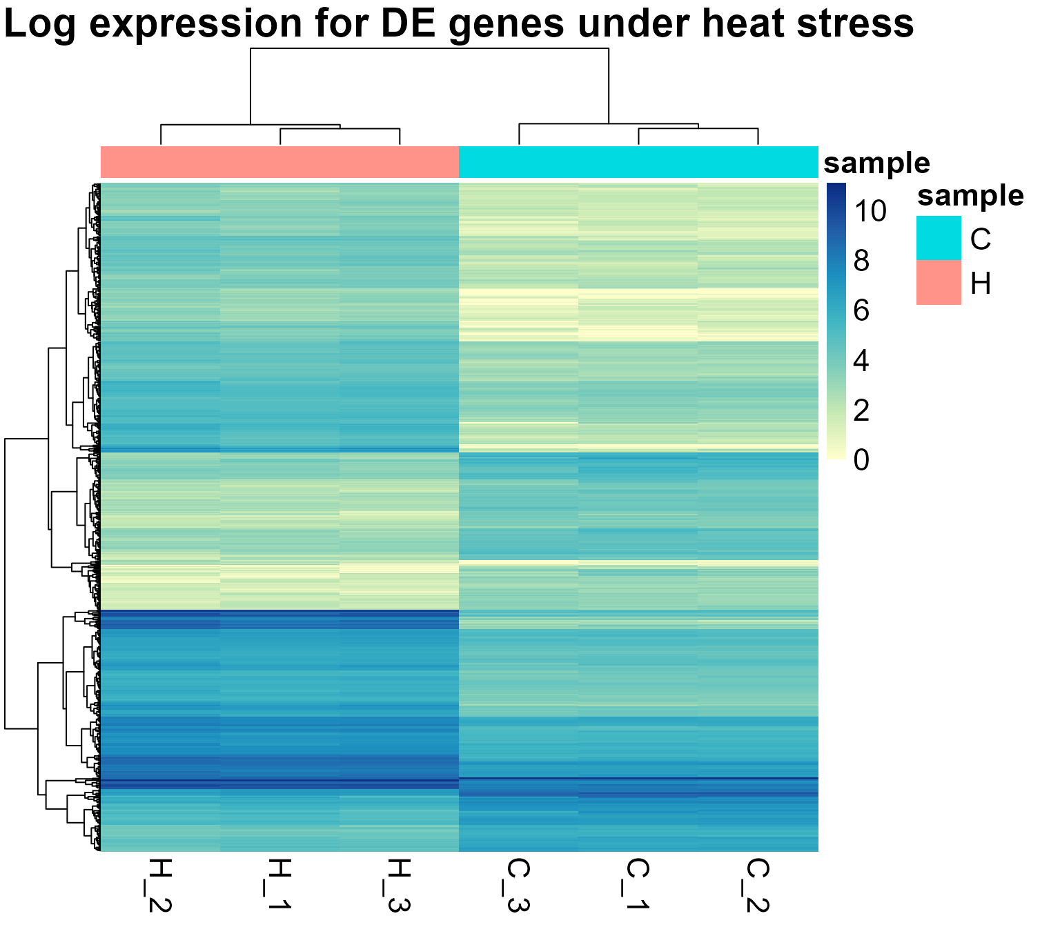
Genes lists comparison
If we want to compare genes differentially expressed between Control and Heat stress, to genes differentially expressed between control and double heat and mannitol stresses :
genes_double_stress <- DIANE::estimateDEGs(fit, reference = "C", perturbation = "MH", p.value = 0.01, lfc = 2)$table$genes

genes_lists <- list("C - H" = genes, "C - HM" = genes_double_stress)
# if we only want the conditions used for differential expression analysis :
DIANE::draw_venn(genes_lists)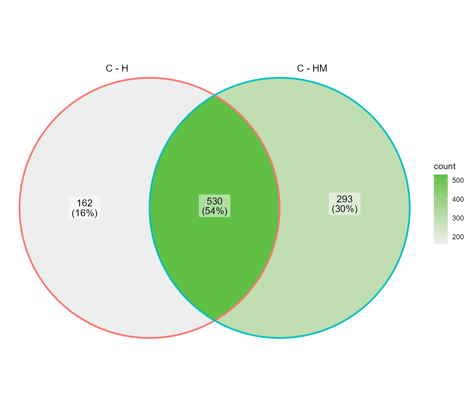
Gene Ontology enrichment analysis
Given any set of genes, we can compute which ontologies are significantly enriched. We compare here our list of heat responsive genes to all the genes present in our expression matrix, referred to as background genes.
If the gene IDs have splicing information (e.g. the transcript number), they must be first transformed to classic AGI terms, with the function get_locus, which is the case here.
The package used behind the enrichment analysis function is clusterProfiler. The method uses Fischer test to detect significant GO terms, and they can be either seen as a result dataframe, or in an interactive plot :
genes <- get_locus(topTags$table$genes)

background <- get_locus(rownames(normalized_counts))

genes <- convert_from_agi(genes)
#>
background <- convert_from_agi(background)


go <- enrich_go(genes, background)
#>
DIANE::draw_enrich_go(go, max_go = 30)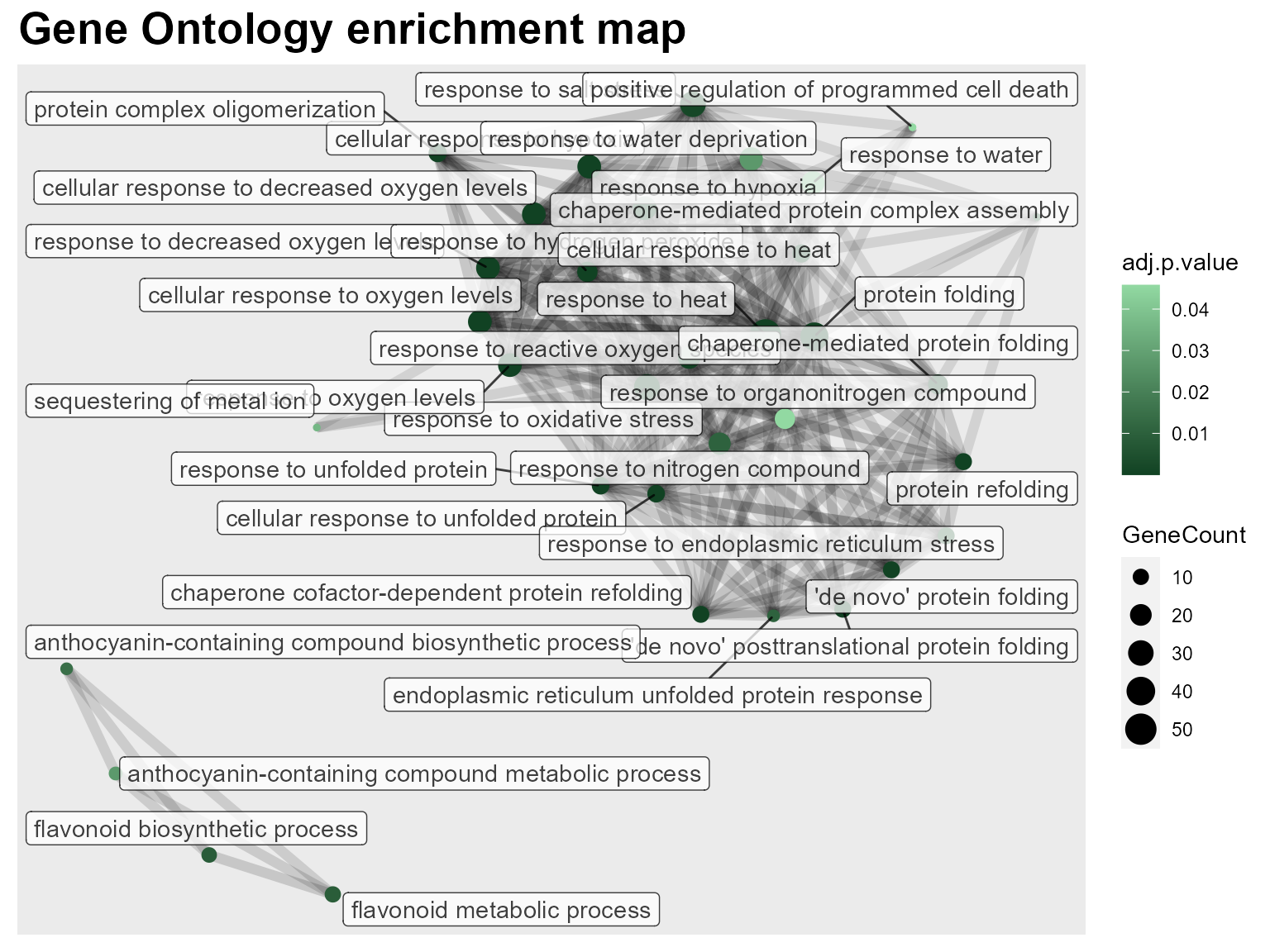
We can limit the number of plotted GO terms with the max go parameter.
As expected, the GO term with the higher gene count is “response to heat”. Then, we also observe GO terms linked to oxygen levels and hypoxia, protein folding and degradation, and responses to various other stresses or compounds.
Expression based clustering
The coseq package relies on the statistical framework of mixture models. Each cluster of genes is represented by a Poisson or Gaussian distribution, which parameters is estimated using Expectation-Maximisation algorithms. In the end of the procedure, the number of clusters that maximizes the clustering quality is chosen.
The input genes of a clustering can’t be all the genes of the data, we use the output of differential expression analysis instead.
You can also specify a subset of the conditions to be used during the clustering if we’re not interested in all the conditions.
Do not forget to use the seed argument to that results can be reproduced.
genes <- topTags$table$genes

clustering <- DIANE::run_coseq(conds = unique(abiotic_stresses$conditions), data = normalized_counts,
                               genes = genes, K = 6:9, transfo = "arcsin", model = "Normal", seed = 123)
#> ****************************************
#> coseq analysis: Normal approach & arcsin transformation
#> K = 6 to 9
#> Use seed argument in coseq for reproducible results.
#> ****************************************
DIANE::draw_coseq_run(clustering$model, plot = "barplots")
#> $probapost_barplots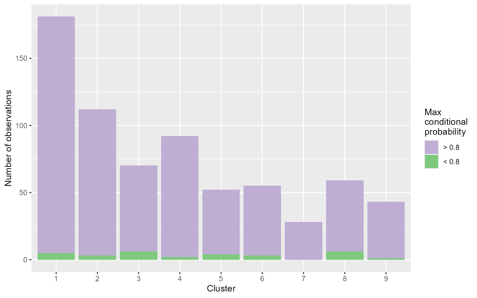
DIANE::draw_coseq_run(clustering$model, plot = "ICL")
#> $ICL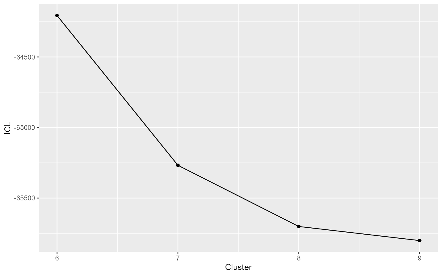
Profiles visualization
The user can display either a view of all the clusters, or focus on one in particular :
DIANE::draw_profiles(data = normalized_counts, clustering$membership, conds = unique(abiotic_stresses$conditions)) 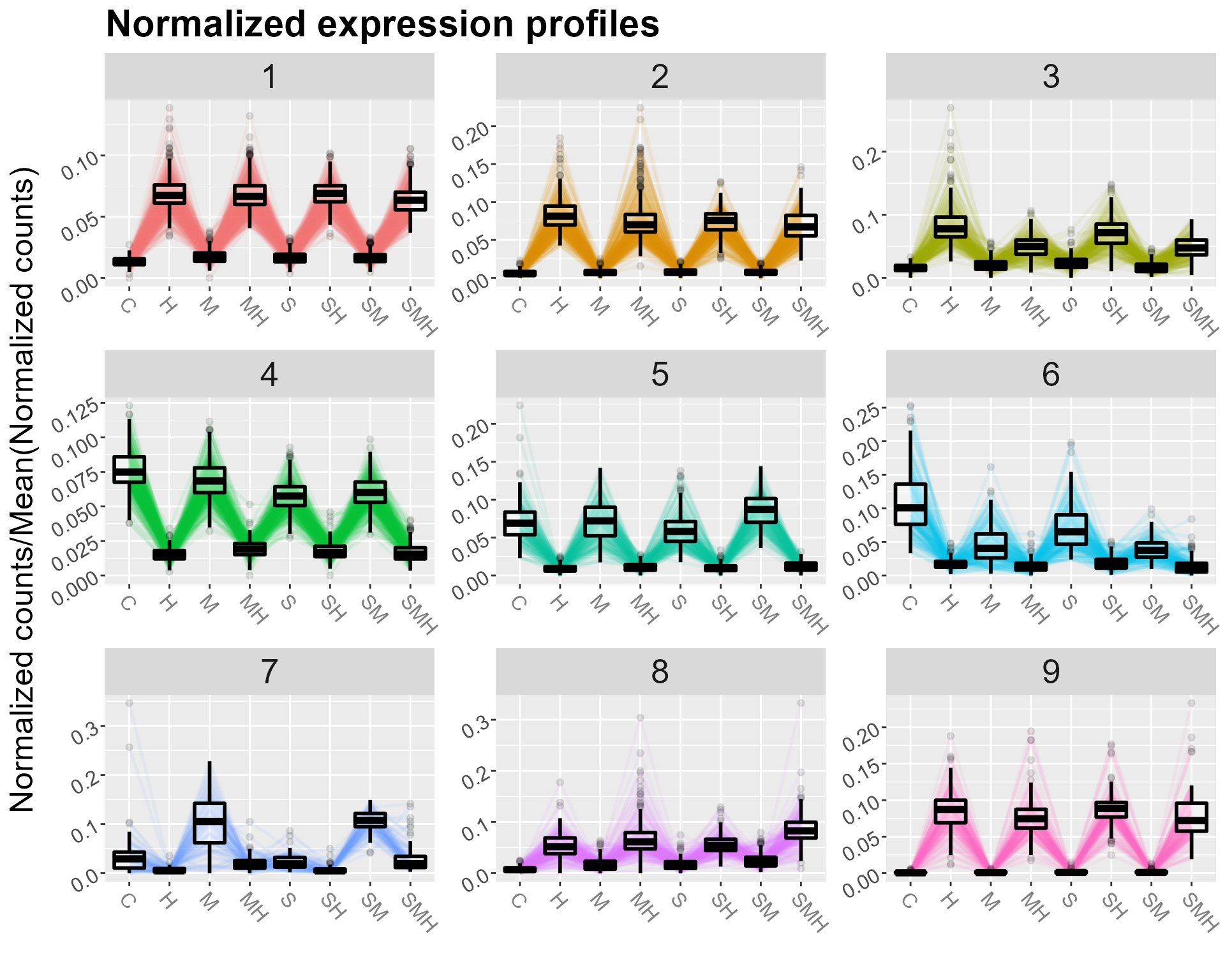
DIANE::draw_profiles(data = normalized_counts, clustering$membership, conds = unique(abiotic_stresses$conditions), k = 3) 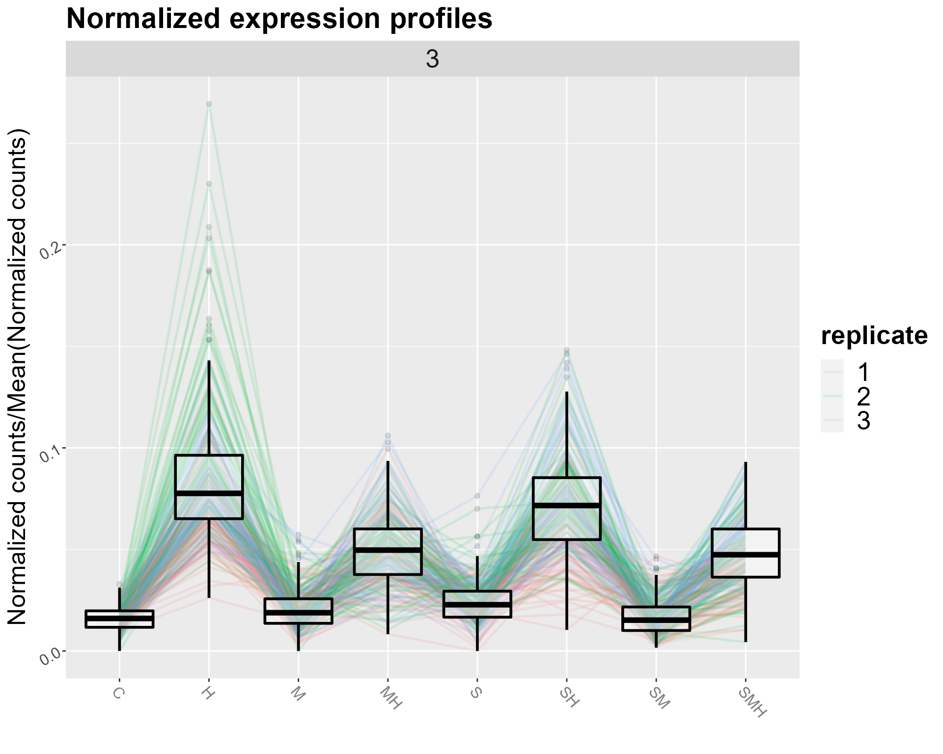
All genes in one cluster can be retrieved with :
DIANE::get_genes_in_cluster(membership = clustering$membership, cluster = 3)
#>  [1] "AT5G50335.1" "AT5G55620.1" "AT1G26800.1" "AT4G04020.1" "AT2G14900.1"
#>  [6] "AT1G54040.2" "AT5G62020.1" "AT5G39190.1" "AT4G28150.1" "AT2G29300.2"
#> [11] "AT3G59350.6" "AT1G73066.1" "AT3G20395.1" "AT5G39160.1" "AT1G21550.1"
#> [16] "AT1G20350.1" "AT1G11960.1" "AT1G66500.1" "AT5G17850.1" "AT1G79780.1"
#> [21] "AT1G47510.1" "AT5G01740.1" "AT2G20880.1" "AT5G15537.1" "AT4G34770.1"
#> [26] "AT5G57760.1" "AT1G65486.3" "AT4G29880.1" "AT5G07380.3" "AT1G06080.1"
#> [31] "AT4G13320.1" "AT1G72760.2" "AT4G28140.1" "AT2G17840.1" "AT3G60670.1"
#> [36] "AT5G61800.1" "AT2G05540.1" "AT3G56090.1" "AT3G26790.1" "AT2G22860.1"
#> [41] "AT1G03010.1" "AT1G70800.1" "AT5G43620.1" "AT3G42800.1" "AT2G18010.1"
#> [46] "AT3G61920.1" "AT2G07655.1" "AT5G53980.1" "AT3G60730.1" "AT3G05790.1"
#> [51] "AT5G01760.1" "AT5G01600.1" "AT1G75750.1" "AT4G15690.1" "AT4G34080.1"
#> [56] "AT2G24535.2" "AT4G24410.1" "AT2G40710.1" "AT1G44830.1" "AT1G33055.1"
#> [61] "AT4G15700.1" "AT3G23510.1" "AT1G52790.1" "AT3G21320.1" "AT5G60310.1"
#> [66] "AT2G44880.2" "AT3G56790.1" "AT4G15680.1" "AT3G20340.1" "AT3G48640.1"
The named vector membership gives, for each gene, its cluster:
head(clustering$membership, n = 40)
#> AT4G12400.2 AT5G48570.1 AT5G12110.1 AT5G64510.1 AT2G19310.1 AT2G29500.1
#>           9           9           9           9           2           9
#> AT4G25200.1 AT1G07350.1 AT3G24100.1 AT2G26150.1 AT3G12050.1 AT5G52640.1
#>           9           2           2           9           1           9
#> AT1G74310.1 AT3G16050.1 AT3G24500.1 AT5G23240.1 AT2G21660.1 AT1G56300.1
#>           2           2           9           2           2           1
#> AT3G46230.1 AT1G72660.1 AT5G12030.1 AT2G32120.1 AT2G46240.1 AT5G25450.1
#>           9           9           9           2           2           9
#> AT1G17460.2 AT1G14360.1 AT1G59860.1 AT1G09140.1 AT1G65040.2 AT1G30070.2
#>           1           1           2           1           1           1
#> AT1G07400.1 AT1G66080.1 AT4G16146.1 AT5G57150.4 AT1G09780.1 AT3G14200.1
#>           9           2           1           2           4           1
#> AT3G25230.2 AT2G20560.1 AT2G25140.1 AT1G01060.1
#>           1           2           1           5
Generalized Poisson regression on a cluster of genes
The idea is to extract the importance and effect of each factor. To do so, the expression of each gene is modeled by a Poisson distribution. The log of its parameter (the expected value) is approximated by a linear combination of the factors in the experiment. The coefficients associated to each factors are estimated to fit gene expression, and can be insightful to characterize genes behavior in a particular cluster. The model with interactions is considered automatically. If your design in not a complete crossed design, the interaction term will be null.
The absolute value of a coefficient gives information about the intensity of its effect on gene expression. The highest coefficient(s) are thus the one(s) having the greater impact on a cluster’s expression profile.
The sign of a coefficient gives information about the way it impacts expression. If it is positive, it increases the expression when the factor is in its perturbation level. If negative, it decreases it.
genes_cluster <- DIANE::get_genes_in_cluster(
clustering$membership, cluster = 3)
glm <- DIANE::fit_glm(normalized_counts, genes_cluster, abiotic_stresses$design)
summary(glm)
#>
#> Call:
#> glm(formula = formula, family = poisson(link = "log"), data = glmData)
#>
#> Deviance Residuals:
#>    Min      1Q  Median      3Q     Max
#> -38.77  -24.24  -17.67  -11.43  385.26
#>
#> Coefficients:
#>                     Estimate Std. Error z value Pr(>|z|)
#> (Intercept)         5.095647   0.005400  943.66   <2e-16 ***
#> Salt                0.480608   0.006870   69.96   <2e-16 ***
#> Mannitol            0.268302   0.007173   37.40   <2e-16 ***
#> Heat                1.595544   0.005922  269.42   <2e-16 ***
#> Salt:Mannitol      -0.643590   0.009784  -65.78   <2e-16 ***
#> Salt:Heat          -0.874392   0.007866 -111.16   <2e-16 ***
#> Mannitol:Heat      -0.985623   0.008336 -118.24   <2e-16 ***
#> Salt:Mannitol:Heat  1.125183   0.011560   97.34   <2e-16 ***
#> ---
#> Signif. codes:  0 '***' 0.001 '**' 0.01 '*' 0.05 '.' 0.1 ' ' 1
#>
#> (Dispersion parameter for poisson family taken to be 1)
#>
#>     Null deviance: 2356223  on 1679  degrees of freedom
#> Residual deviance: 2179966  on 1672  degrees of freedom
#> AIC: 2189654
#>
#> Number of Fisher Scoring iterations: 7

draw_glm(glm)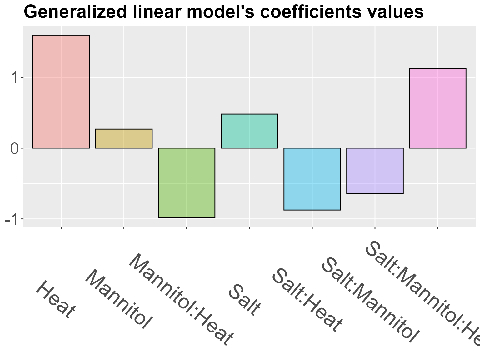
Network inference
We want to build a Gene Regulatory Network, a graph connecting regulator genes to any other genes (targets or other regulators).
Regulators for your organism
A list of regulators are provided in DIANE for a number of model organisms. For example, here are the ones for Human and Arabidopsis :
print(head(regulators_per_organism[["Arabidopsis thaliana"]]))
#> [1] "AT1G04880" "AT1G20910" "AT1G55650" "AT1G76110" "AT1G76510" "AT2G17410"
print(head(regulators_per_organism[["Homo sapiens"]]))
#> [1] "ENSG00000004848" "ENSG00000005073" "ENSG00000005102" "ENSG00000005513"
#> [5] "ENSG00000005801" "ENSG00000005889"
If your gene IDs are splicing aware, this is not of any use to the inference method, so we want to aggregate the data first. For each gene, we sum all its transcripts to have the final expression levels.
aggregated_data <- aggregate_splice_variants(data = normalized_counts)Inference and visualization
The inference can now be performed.
Classic GENIE3 inference
Network inference takes as input a list of genes, generated by differential expression tests, that will be the nodes of the inferred network. Among those genes, some must be identified as potential transcriptional regulators. It is also possible to use a subset of genes for network inference, as clusters determined in the expression based clustering tab.
The GENIE3 package is a method based on Machine Learning (Random Forests) to infer regulatory links between target genes and regulator genes. The advantages of this method is that it returns oriented edges from regulators to targets, which is desired in the context of regulatory networks, and can capture high order interactions between regulators.
For each target gene, the methods uses Random Forests to provide a ranking of all regulators based on their influence on the target expression. This ranking is then merged across all targets, giving a global regulatory links ranking. Settings relative to regulatory weights inference are presented in the left pane.
The idea is then to keep the strongest links to build the gene regulatory network. The way of determining the right number of final edges in the network can be based on a desired network density alone, or followed by edges statistical testing.
Again, we set the seed before using the network inference procedure which is based on random processes :
set.seed(123)
mat <- DIANE::network_inference(grouped_counts, conds = abiotic_stresses$conditions,
                                targets = grouped_targets, regressors = grouped_regressors,
                                nCores = 1, verbose = FALSE)

network <- DIANE::network_thresholding(mat, n_edges = length(genes))

data <- network_data(network, regulators_per_organism[["Arabidopsis thaliana"]],
                     gene_annotations$`Arabidopsis thaliana`)

knitr::kable(head(data$nodes))| id | label | degree | community | group | gene_type | description | |
|---|---|---|---|---|---|---|---|
| AT1G07900 | AT1G07900 | LBD1 | 30 | 1 | Regulator | Regulator | LOB domain-containing protein 1 |
| mean_AT5G24110-AT3G12910-AT2G37430-AT5G56960 | mean_AT5G24110-AT3G12910-AT2G37430-AT5G56960 | mean_WRKY30-AT3G12910-ZAT11-AT5G56960 | 37 | 2 | Grouped Regulators | Grouped Regulators | NA |
| AT3G23230 | AT3G23230 | TDR1 | 34 | 2 | Regulator | Regulator | encodes a member of the ERF (ethylene response factor) subfamily B-3 of ERF/AP2 transcription factor family. The protein contains one AP2 domain. There are 18 members in this subfamily including ATERF-1, ATERF-2, AND ATERF-5. |
| mean_AT1G17460-AT5G57150-AT5G60100-AT5G48250-AT1G09530-AT3G62090-AT1G11100-AT5G39610-AT3G11020-AT1G67370-AT1G74890 | mean_AT1G17460-AT5G57150-AT5G60100-AT5G48250-AT1G09530-AT3G62090-AT1G11100-AT5G39610-AT3G11020-AT1G67370-AT1G74890 | mean_TRFL3-AT5G57150-PRR3-BBX8-PIF3-PIL2-FRG5-NAC6-DREB2B-ASY1-ARR15 | 73 | 3 | Grouped Regulators | Grouped Regulators | NA |
| AT5G22570 | AT5G22570 | WRKY38 | 32 | 1 | Regulator | Regulator | member of WRKY Transcription Factor |
| AT2G40750 | AT2G40750 | WRKY54 | 29 | 1 | Regulator | Regulator | member of WRKY Transcription Factor |
DIANE::draw_network(data$nodes, data$edges)network is an igraph object, and can be analyzed with all the possibilities offered by this complete package about graphs algorithms.
DIANE’s edges testing procedure
A matrix of importances is computed, just as in the previous section, but we prefer to use another importance metric for consistency reasons.
set.seed(123)
mat <- DIANE::network_inference(grouped_counts,
                                conds = abiotic_stresses$conditions,
                                targets = grouped_targets,
                                regressors = grouped_regressors,
                                importance_metric = "MSEincrease_oob",
                                verbose = TRUE)
Then, we are going to generate a first network, by considering only the number of pairs offering a state of the art density value. The density is usually between 0.1 and 0.001, as reviewed in several papers about biological network topology. This step is crucial, as it prevents from testing all possible pairs, which would be useless for a huge majority of pairs, as well as extremely costly.
nGenes = length(grouped_targets)
nRegulators = length(grouped_regressors)

res <- data.frame(density = seq(0.001, 0.1, length.out = 20),
                  nEdges = sapply(seq(0.001, 0.1, length.out = 20),
                                  get_nEdges, nGenes, nRegulators))
ggplot(res, aes(x = density, y = nEdges)) + geom_line(size = 1) +
  ggtitle("Number of network edges as a function of its density") +
  geom_vline(xintercept = 0.03, color = "darkgreen", lty = 2, size = 1.2)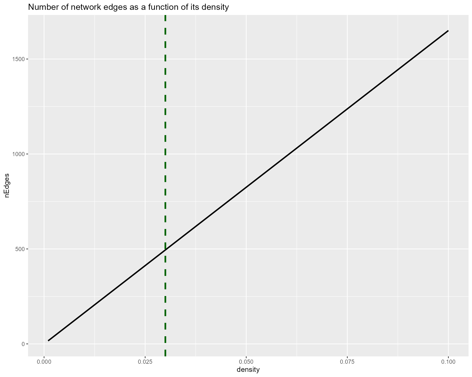
Given this graph, we can consider that a density value of 0.03 would be a good compromise between a small enough subset of edges to test, and a coherent density value, not too restrictive. This step will take a certain time to run, from a few minutes to tens of minutes depending on your hardware.
set.seed(123)
res <- DIANE::test_edges(mat, normalized_counts = grouped_counts, density = 0.03,
                         nGenes = nGenes,
                         nRegulators = nRegulators,
                         nTrees = 1000, verbose = TRUE)
The elements contained in the result variable are the network edges associated to their adjusted pvalue, as well as graphics to guide the user in the choice of the adjusted pvalue (fdr) threshold to use for the final network.
res$fdr_nEdges_curve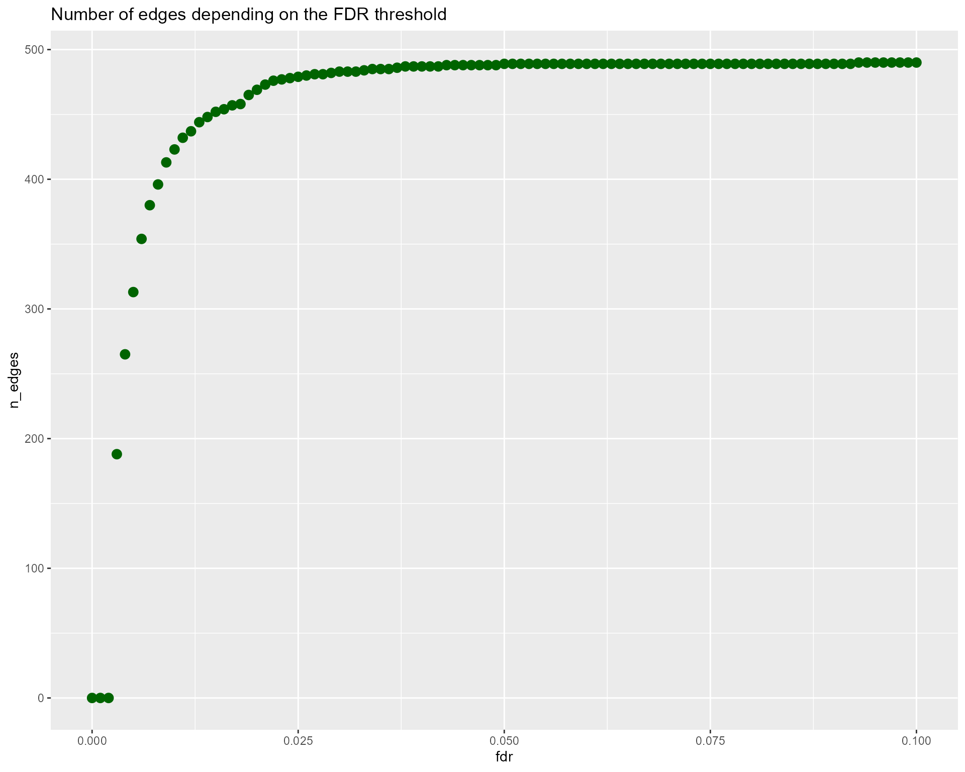
res$pvalues_distributions + xlim(0,0.1)
#> Scale for 'x' is already present. Adding another scale for 'x', which will
#> replace the existing scale.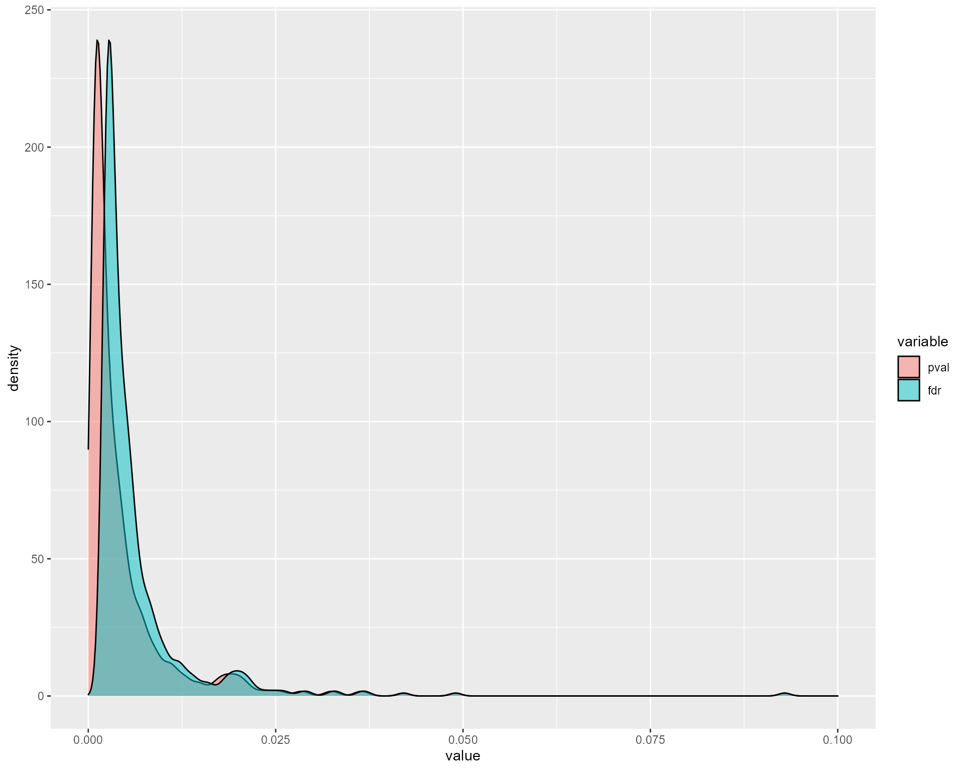
kable(head(res$links))| regulatoryGene | targetGene | pval | fdr |
|---|---|---|---|
| AT1G07900 | AT3G15534 | 0.000999 | 0.0026038 |
| mean_AT2G20880-AT4G28140 | AT3G15534 | 0.048951 | 0.0490512 |
| mean_AT1G14580-AT2G18328-AT1G19510-AT3G14740-AT5G59570 | AT3G15534 | 0.041958 | 0.0421300 |
| mean_AT2G26150-AT3G24500-AT4G11660-AT4G34530-AT1G73830-AT3G46640-AT5G05410-AT1G22190-AT3G26790-AT5G62020-AT3G23150-AT3G60670 | AT1G75040 | 0.001998 | 0.0036944 |
| AT3G23230 | AT1G75040 | 0.000999 | 0.0026038 |
| mean_AT1G01060-AT1G20693 | AT1G75040 | 0.009990 | 0.0112016 |
net <- DIANE::network_from_tests(res$links, fdr = 0.05)
#> 489 edges kept in final network
All right, the network is ready to be analyzed!
Visualization
The first graph shows, in red, the edges that were not significant according to our perumtation tests.
net_data <- network_data(net, regulators_per_organism[["Arabidopsis thaliana"]], gene_annotations$`Arabidopsis thaliana`)
draw_discarded_edges(res$links, net_data)
#> 490 edges kept in final network
The second graph shows to final infered network :
draw_network(net_data$nodes, net_data$edges)A community discovery is performed using the Louvain algorithm, so we can extract highly connected genes modules. You can see those communities on the graph and plot their profiles:
data$nodes$group <- data$nodes$community

louvain_membership <- data$nodes$community
names(louvain_membership) <- data$nodes$id

knitr::kable(head(louvain_membership, n = 10))| x | |
|---|---|
| AT1G07900 | 1 |
| mean_AT5G24110-AT3G12910-AT2G37430-AT5G56960 | 2 |
| AT3G23230 | 2 |
| mean_AT1G17460-AT5G57150-AT5G60100-AT5G48250-AT1G09530-AT3G62090-AT1G11100-AT5G39610-AT3G11020-AT1G67370-AT1G74890 | 3 |
| AT5G22570 | 1 |
| AT2G40750 | 1 |
| AT1G44830 | 2 |
| mean_AT1G01060-AT1G20693 | 2 |
| AT3G22100 | 4 |
| mean_AT2G26150-AT3G24500-AT4G11660-AT4G34530-AT1G73830-AT3G46640-AT5G05410-AT1G22190-AT3G26790-AT5G62020-AT3G23150-AT3G60670 | 5 |
DIANE::draw_network(data$nodes, data$edges)
draw_profiles(aggregated_data, membership = louvain_membership, conds = abiotic_stresses$conditions)
#> Warning: Removed 168 rows containing non-finite values (stat_boxplot).
#> Warning: Removed 168 row(s) containing missing values (geom_path).
#> Warning: Removed 168 rows containing missing values (geom_point).
Gene ontology enrichment can also be performed on gene communities (However, if there is too few genes, GO enrichment tests may not be significant).
Analysis
We can plot the network connectivity statistics, and get the regulators and targets of a gene as follows :
DIANE::draw_network_degrees(net_data$nodes, net)
#> `stat_bin()` using `bins = 30`. Pick better value with `binwidth`.
#> `stat_bin()` using `bins = 30`. Pick better value with `binwidth`.
#> `stat_bin()` using `bins = 30`. Pick better value with `binwidth`.
#> `stat_bin()` using `bins = 30`. Pick better value with `binwidth`.
nodes <- data$nodes[order(-data$nodes$degree),]
gene_of_interest <- nodes$id[1]

print(DIANE::describe_node(network, node = gene_of_interest))
#> $targets
#>  [1] "AT1G44830" "AT5G53980" "AT2G34440" "AT1G72920" "AT3G48640" "AT1G56240"
#>  [7] "AT4G12490" "AT5G57760" "AT3G56790" "AT3G20340" "AT2G21650" "AT5G39670"
#> [13] "AT5G50335" "AT1G22690" "AT3G20395" "AT2G14900" "AT5G55620" "AT4G19430"
#> [19] "AT4G15680" "AT1G73066" "AT3G23510" "AT3G21320" "AT4G37400" "AT1G47480"
#> [25] "AT3G01960" "AT2G28560" "AT3G25180" "AT5G01740" "AT3G56090" "AT4G15690"
#> [31] "AT4G18205" "AT5G05250" "AT3G42800" "AT1G54040" "AT4G12495" "AT1G75750"
#> [37] "AT2G14610" "AT1G52790" "AT1G80660" "AT3G53250" "AT1G26800" "AT5G54720"
#> [43] "AT5G41590" "AT4G13320" "AT4G34770" "AT2G24535" "AT2G17840" "AT5G54710"
#> [49] "AT5G44565" "AT2G21640" "AT3G28220" "AT2G35850" "AT4G29880" "AT1G44970"
#> [55] "AT3G45130" "AT5G60310" "AT2G22860" "AT5G54165" "AT1G06080" "AT1G21550"
#> [61] "AT3G60730" "AT2G21840" "AT4G07995" "AT4G12500" "AT5G01600" "AT1G65486"
#> [67] "AT3G03910" "AT4G13410" "AT4G34510" "AT4G24410" "AT3G61920" "AT1G13420"
#> [73] "AT4G01335" "AT1G03010" "AT4G01630" "AT5G43620" "AT2G35960" "AT1G70800"
#> [79] "ATMG00640" "AT1G71000" "AT3G25100" "AT4G24413" "AT1G09350" "AT1G76994"
#> [85] "AT3G44753" "AT2G29300"
#>
#> $regulators
#> character(0)